Introduction — The Search Engine That Gets Its Priorities Wrong

Imagine you’re looking for a freelance contract.

You type:

React Senior Paris

Your search engine—powered by embeddings, modern, supposedly intelligent—returns this:

1. React Junior Lyon          ← ??
2. React Senior Brussels      ← close, but not Paris
3. React Fullstack Paris      ← Paris, but not Senior
4. React Senior Paris         ← exactly what you wanted — in 4th place

You look at the results and wonder what’s going on.

The engine is using vector embeddings. It knows that « React » is related to frontend development, that « Paris » is a city, and that « Senior » implies experience. Conceptually, it understands the domain.

So why is the best result only fourth?

This isn’t a bug. It’s a fundamental architectural limitation of Dense Retrieval.

To understand—and fix—it, we first need to understand how embeddings actually work, where their limitations lie, and why modern RAG systems almost always rely on a two-stage pipeline:

Retrieve → Re-rank

1. Dense Retrieval — The Bi-Encoder

The Principle Behind Embeddings

An embedding is simply the transformation of a piece of text into a vector of numbers.

"React Senior Paris" → [0.23, -0.87, 0.41, 0.66, ...]
                        (384 or 768 dimensions)

This vector captures the overall meaning of the text. Two semantically similar texts produce vectors that are close to each other in vector space.

That’s the promise of embeddings: capturing meaning, not just words.

The Bi-Encoder

A Bi-Encoder is the model that produces these embeddings.

It encodes the query and each document independently:

          QUERY                       DOCUMENT
            |                             |
    ┌────────────────┐          ┌────────────────┐
    │  Transformer   │          │  Transformer   │
    │  (Bi-Encoder)  │          │  (Bi-Encoder)  │
    └────────────────┘          └────────────────┘
            |                             |
         Vector A                      Vector B
            |                             |
            └──────────┬──────────────────┘
                       |
               Cosine Similarity
                       |
                     Score

Both texts go through the same model, but completely independently.

Why It’s Fast

This is the key to everything.

Document embeddings are computed only once, during indexing. They’re then stored in a Vector Database such as Qdrant, Pinecone, or Weaviate.

At query time, only the query embedding is computed in real time. That vector is then compared against all the stored vectors.

INDEXING (one-time operation)
─────────────────────────────────────────────
Document 1 → Embedding → stored
Document 2 → Embedding → stored
Document 3 → Embedding → stored
...
10 million documents → 10M stored vectors


QUERY (real time)
─────────────────────────────────────────────
"React Senior Paris"
         |
    Bi-Encoder
         |
      Vector Q
         |
    Vector Search
 (ANN - Approximate Nearest Neighbors)
         |
    Top 50 results
   in a few milliseconds

Even with 10 million documents, vector search can retrieve the top 50 candidates in just a few milliseconds. That’s what makes Vector Databases practical at scale.

Cosine Similarity — The Intuition

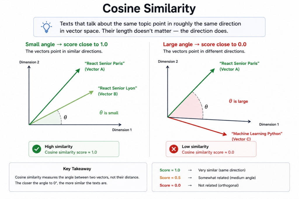
Cosine Similarity measures the angle between two vectors, not their distance.

The intuition is simple: texts discussing the same topic tend to point in roughly the same direction in vector space. Their length doesn’t matter—the direction does.

2. The Limitations of Dense Retrieval — The Real Problem

This is where things become more complicated.

Semantics Are Global, Not Precise

A Bi-Encoder captures the general meaning of a text. It understands topics, domains, and overall context.

But it does not compare texts word by word.

As a result, semantically similar texts can end up with similar embeddings even when they differ on the details that actually matter.

A Concrete Example — Job Search

Query:

React Senior Paris

Documents:

A: "React Junior Lyon"
B: "React Senior Brussels"
C: "React Fullstack Paris"
D: "React Senior Paris"

From the embedding model’s perspective:

« React » appears in all four documents.
« Senior » versus « Junior » is only a subtle semantic distinction.
« Paris », « Lyon », and « Brussels » are all city names and therefore semantically related.

The model sees four frontend job offers in similar domains. It does not ask:

« Does this document exactly match the query? »

Instead, it asks:

« Do these two vectors point in roughly the same direction? »

That’s a fundamentally different question.

The Key Takeaway

Vector similarity is an approximation of general meaning.

It’s excellent at quickly finding documents that talk about the right topic.

It’s much worse at distinguishing documents that discuss the same topic but differ on important details.

It’s an approximation of relevance—not relevance itself.

3. The Cross-Encoder — Reading Both Texts Together

The Fundamental Difference

A Bi-Encoder encodes the query and the document separately.

A Cross-Encoder reads them together.

BI-ENCODER
──────────────────────────────────────────────
Query      →  Transformer  →  Vector A
                                         →  Cosine Similarity  →  Score
Document   →  Transformer  →  Vector B


CROSS-ENCODER
──────────────────────────────────────────────
[Query + Document]
          |
     Transformer
          |
   Relevance Score (0 → 1)

This isn’t an implementation detail. It’s a completely different paradigm.

Why Seeing Both Texts Together Changes Everything

With a Bi-Encoder:

"React Senior Paris"   →   vector [0.23, -0.87, 0.41, ...]
"React Junior Lyon"    →   vector [0.21, -0.84, 0.39, ...]

These vectors are close to each other.

The model never had the opportunity to compare the two texts directly. It simply encoded each one independently.

With a Cross-Encoder:

Input: "[CLS] React Senior Paris [SEP] React Junior Lyon [SEP]"
         |
  Transformer with Attention
         |
   Score: 0.31 (low relevance)

Input: "[CLS] React Senior Paris [SEP] React Senior Paris [SEP]"
         |
  Transformer with Attention
         |
   Score: 0.97 (high relevance)

The model reads the query in direct relation to the document. Every word in the query can interact with every word in the document.

The Role of Attention — The Intuition

The Attention mechanism (Transformer Self-Attention) allows every word in a text to « look at » every other word in order to understand its context.

In a Cross-Encoder, this mechanism operates on both texts combined.

Query:      React  Senior  Paris
               ↕      ↕      ↕
Document:   React  Junior  Lyon

The model can directly compare:

« Senior » in the query with « Junior » in the document → they are different.
« Paris » in the query with « Lyon » in the document → they are different.

It doesn’t compare global vectors anymore. It analyzes the relationships between words across both texts.

That’s why Cross-Encoders are dramatically more accurate.

4. Why Cross-Encoders Are Slow

The Problem with On-the-Fly Computation

With a Bi-Encoder, document embeddings are precomputed.

With a Cross-Encoder, nothing can be precomputed.

The score depends on the pair (query, document). Until the query is known, no computation can be performed.

For every new query, you need to run a full Transformer inference for every document.

The Cost Explodes

100 documents       →      100 Transformer inferences      → ~1 second
1,000 documents     →    1,000 Transformer inferences      → ~10 seconds
100,000 documents   →  100,000 Transformer inferences      → ~17 minutes
10,000,000 docs     →   10M Transformer inferences         → IMPOSSIBLE

Transformer inference isn’t cheap. A standard Cross-Encoder such as BERT-base takes roughly 5–10 ms per query-document pair on a GPU.

For 10 million documents, that’s 14 to 28 hours per query.

Completely impractical.

5. The Modern Solution — The Retrieve → Re-rank Pipeline

The Best of Both Worlds

The solution is elegant: use both models in sequence.

10,000,000 documents
         |
    ─────────────────
     Dense Retrieval
       (Bi-Encoder)
    ─────────────────
         |
     Top 50 candidates
      (a few ms)
         |
    ─────────────────
        Re-ranking
     (Cross-Encoder)
    ─────────────────
         |
      Top 5 results
     (high precision)
         |
          LLM
         |
     Final answer

Why It Works

Dense Retrieval solves the scalability problem: it quickly finds the 50 most likely relevant documents out of millions.

The Cross-Encoder solves the precision problem: it re-ranks those 50 documents using a much finer understanding of actual relevance.

STEP 1 — Dense Retrieval
────────────────────────────────────────────────────
Goal        : "Find plausible candidates"
Speed       : Milliseconds
Precision   : Approximate
Scale        : 10 million documents → Top 50
Model        : Bi-Encoder (precomputed vectors)


STEP 2 — Re-ranking
────────────────────────────────────────────────────
Goal        : "Rank candidates precisely"
Speed       : ~250 ms for 50 documents
Precision   : High
Scale        : 50 documents → Top 5
Model        : Cross-Encoder (on-the-fly inference)

Running 50 Cross-Encoder inferences takes around 250 to 500 ms, which is perfectly acceptable.

The Logic Behind the Pipeline

Dense Retrieval doesn’t need to find the right answers.

It needs to avoid missing them.

Its job is to ensure that the top 50 candidates contain the truly relevant documents, even if their internal ranking isn’t perfect.

The Cross-Encoder then takes care of putting those candidates in the right order.

6. A Real-World Example — mission-radar-ai

Imagine a platform that analyzes LinkedIn job opportunities and ranks them according to a freelancer’s profile.

The Profile

Freelance Developer
- Skills       : Python, FastAPI, LangChain, React
- Experience   : Senior (10 years)
- Preference   : Fully remote
- Contract type: Engagements longer than 6 months

The Available Opportunities

Opportunity A: "Senior Python Developer - Remote - 6 months - Paris"
Opportunity B: "Junior Python Developer - On-site - 3 months - Lyon"
Opportunity C: "Python Architect - Remote - 12 months - Toulouse"
Opportunity D: "Senior React Developer - Remote - 6 months - Bordeaux"
Opportunity E: "Senior Python Developer - Remote - 6 months - Paris"

Step 1 — Dense Retrieval

The profile is transformed into an embedding.

Vector search returns the five opportunities, probably in this order:

1. Opportunity E : score 0.94 (almost identical)
2. Opportunity A : score 0.93 (very close)
3. Opportunity C : score 0.91 (Python, Remote, but Architect)
4. Opportunity D : score 0.88 (Senior, Remote, but React)
5. Opportunity B : score 0.81 (Python, but Junior + On-site)

The ranking is already reasonable, but:

Opportunity C (Architect, 12 months) is probably a better fit than Opportunity D.
Opportunity B (Junior) shouldn’t really be there.

Step 2 — Cross-Encoder

The Cross-Encoder re-evaluates every (profile, opportunity) pair:

CrossEncoder("[full profile] [SEP] Opportunity E") → 0.97
CrossEncoder("[full profile] [SEP] Opportunity A") → 0.94
CrossEncoder("[full profile] [SEP] Opportunity C") → 0.89
CrossEncoder("[full profile] [SEP] Opportunity D") → 0.72
CrossEncoder("[full profile] [SEP] Opportunity B") → 0.18

Final ranking:

1. Opportunity E (0.97) — Senior Python, Remote, 6 months, Paris ✓
2. Opportunity A (0.94) — Senior Python, Remote, 6 months, Paris ✓
3. Opportunity C (0.89) — Python Architect, Remote, 12 months ✓
4. Opportunity D (0.72) — Senior React, Remote ~
5. Opportunity B (0.18) — Junior Python, On-site ✗

The Cross-Encoder correctly identified that Opportunity B is a poor match because it’s both junior-level and on-site, giving it a score of only 0.18.

These top results can then be sent to an LLM to generate a structured response: analysis, strengths, weaknesses, and recommendations.

7. When This Pipeline Really Makes a Difference

This pipeline is particularly valuable when:

Selection Criteria Are Precise and Conjunctive

Job search, real estate, and e-commerce often involve multiple filters (location + seniority + contract type).

If the result needs to satisfy several criteria simultaneously, Dense Retrieval alone is usually not enough.

The Corpus Is Large and Heterogeneous

Beyond 100,000 documents, the quality of pure Dense Retrieval tends to degrade.

Re-ranking compensates for this loss of precision.

The Query Is Nuanced

« An article about the risks of Deep Learning, not its benefits. »

A Bi-Encoder may struggle with the negation.

A Cross-Encoder analyzes the relationship between the query and the document and is much better at capturing this kind of nuance.

The Cost of a Bad Answer Is High

Medical, legal, or financial recommendation systems often require a higher level of precision.

In these cases, the additional latency introduced by a Cross-Encoder is usually worth it.

8. Recommended Resources

Sentence Transformers — Retrieve & Re-rank

https://sbert.net/examples/applications/retrieve_rerank

The reference implementation.

The Sentence Transformers repository provides a complete Retrieve → Re-rank pipeline with pre-trained models. The code is easy to follow and the examples are straightforward.

Read this if: you want to implement the pipeline quickly in Python.

The documentation also recommends models for each stage, including the popular ms-marco-MiniLM rerankers.

Sentence Transformers — Cross Encoders

https://sbert.net/docs/package_reference/cross_encoder

The technical documentation for Cross-Encoders in the Sentence Transformers library.

It shows how to load a model, score query-document pairs, and integrate a Cross-Encoder into an existing pipeline.

Read this if: you’ve understood the theory and want to move on to implementation.

Hugging Face — Training Rerankers

https://huggingface.co/learn/cookbook/en/training_rerankers

A practical guide to fine-tuning your own Cross-Encoder for a specific domain.

It explains the required training data (query-document pairs with relevance labels) and walks through the entire process.

Read this if: the generic models are no longer sufficient and you need a domain-specific reranker for job listings, technical documentation, legal documents, and so on.

Weaviate — Cross Encoders as Rerankers

https://weaviate.io/blog/cross-encoders-as-rerankers

A great article explaining how re-ranking can be integrated directly into a Vector Database.

Read this if: you’re working with Weaviate or simply want a better understanding of how modern vector databases increasingly support reranking natively.